WRF V3.1을 미국 지역에 적용해 보기

WRF ARW V3.1 설치기를 보고 설치에 성공하였다면,
다음은 미국 지역에 실제로 적용해 보도록 하겠습니다.
(January 2000 Case)
참고) 우리나라 주변 지역의 설정에 관해서는 개인적으로 연락 주시기 바랍니다. ^-^.

모형에 사용될 입력자료를 준비하기 위하여 WPS 디렉토리로 이동한다.
```
%cd WPS
```

“namelist.wps"를 편집하여 다음을 수정한다.

max_dom = 1
parent_id = 1,
parent_grid_ratio = 1,
i_parent_start = 1,
j_parent_start = 1,
e_we = 74,
e_sn = 61,
geog_data_res = '10m',
dx = 30000,
dy = 30000,
map_proj = 'lambert',
ref_lat = 34.83,
ref_lon = -81.03,
stand_lon = -98.0,
geog_data_path = 'terrestrial 자료가 있는 디렉토리 위치'

제대로 설정되었는지를 “./util/plotgrids.exe"를 실행하여 “gmeta"가 생성되면,
NCAR Graphics의 idt 명령으로 다음과 같은 그림을 확인한다.
```
%idt gmeta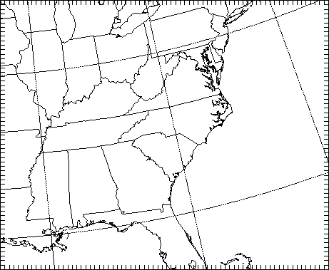
```
“./geogrid.exe"를 실행하고 “geo_em.d01.nc” 가 생성되었으면, ncview 등으로 화면상으로 확인하거나, “ncdump -h geo_em.d01.nc"의 명령으로 내용을 텍스트로 직접 확인해 본다.
1월달의 입력자료를 여기에서 가져와서 data 디렉토리 아래에 풀어준다.
```
%cd ../data; tar xvzf JAN00.tar.gz
```
이 자료는 WPS 디렉토리의 util/g1print.exe로 간략한 내용들을 볼 수 있다.
```
%cd ../WPS; ./util/g1print.exe ../data/JAN00/2000012412.AWIPSF
```
AWIP 자료이므로 AWIP Vtable을 링크하고 GRIB 자료들을 링크한다.
```
%ln -sf ungrib/Variable_Tables/Vtable.AWIP Vtable
%./link_grib.csh ../data/JAN00/2000012*
```
그러면, Vtable과 GRIBFILE.AAA, GRIBFILE.AAB, …. 등이 모두 링크되었을 것이다.
ungrib을 실행하기 위하여 namelist.wps를 다음과 같이 수정하고,
```
start_date = '2000-01-24_12:00:00',
end_date = '2000-01-25_12:00:00',
interval_seconds = 21600,
prefix = 'FILE',
```
다음과 같이 실행하면 “FILE:2000-01-24_12”, “FILE:2000-01-24_18” 등의 입력 자료가 생성된다.
```
%./ungrib.exe >& ungrib_data.log
```

자료를 확인하기 위해서 다음의 두 가지 방법으로 테스트 해 본다.

%./util/rd_intermediate.exe FILE:2000-01-24_12
%./util/plotfmt.exe FILE:2000-01-24_12 ; idt gmeta

metgrid에는 namelist.wps에서 특별하게 설정한 것이 없으니 바로 실행한다.
```
%./metgrid.exe
```
실행 후에는 met_em.d01.2000-01-24_??:??:??.nc 화일이 생성되므로
ncview 또는 ncdump -h 로 확인해 본다.
입력자료가 모두 생성되었으므로 WRF를 실행하기 위하여 WRFV3 디렉토리로 이동하고
입력 자료를 링크한다.
```
%cd ../WRFV3/test/em_real
%ln -sf ../../../WPS/met_em.d01.2000-01* .
```

namelist.input를 다음과 같이 수정하고 real.exe를 실행한다.

run_days = 0,
run_hours = 12,
run_minutes = 0,
run_seconds = 0,
start_year = 2000,
start_month = 01,
start_day = 24,
start_hour = 12,
end_year = 2000,
end_month = 01,
end_day = 25,
end_hour = 12,
interval_seconds = 21600
input_from_file = .true.,
history_interval = 180,
max_dom = 1,
s_we = 1,
e_we = 74,
s_sn = 1,
e_sn = 61,
s_vert = 1,
e_vert = 28,
num_metgrid_levels = 27
dx = 30000,
dy = 30000,

%real.exe 를 실행한 후 생성되는 wrfinput_d01과 wrfbdy_d01을 ncview 또는 ncdump -h 로 확인해 본다.

이제 모든 준비가 다 되었으므로 wrf를 실행한다.
```
%wrf.exe
```
실행이 끝나면, “wrfout_d01_2000-01-24_12:00:00 등이 생성되므로 이것으로 분석을 하면 된다.
```
%ncdump -h wrfout_d01_2000-01-24_12:00:00
%ncdump -v Times wrfout_d01_2000-01-24_12:00:00 --> 모의 시간을 볼 수 있다.
%ncview wrfout_d01_2000-01-24_12:00:00
```
Good luck !

#수치모형 #대기순환모형 #WRF